Each model builds on the limitations of the previous one. The results below come from training and evaluating all three on the Titanic dataset using identical preprocessing and splits.
A single model that learns to split data by asking yes or no questions at each node. It picks the feature and threshold that best separates the classes at each step. Fast to train and easy to visualize, but it tends to memorize training data rather than learn general patterns.
G = 0 is a perfectly pure node. Every split picks the threshold that minimizes the weighted Gini of the two children.
Bootstrap Aggregating trains many separate trees, each on a different random sample of the training data drawn with replacement. Final predictions come from a majority vote or average across all trees. Every tree still has access to all features at every split.
= 1 − (890/891)891
Var(T̅B) = ρσ2 + (1 − ρ)σ2 / B
ρ is the pairwise correlation between trees. The ρσ2 term is a hard floor. Adding more trees never removes it. Only reducing ρ does. That is exactly what random forests target.
Like bagging but with one critical addition. At each node split, only a random subset of features is considered rather than all of them. This prevents any single strong feature from dominating every tree, making the trees genuinely different from each other and the ensemble far more powerful.
Bagging: ρ ≈ 0.76 → floor = 0.76 σ2
RF: ρ ≈ 0.67 → floor = 0.67 σ2
Forcing each split to consider only m features stops dominant features from appearing in every tree. Cutting ρ from 0.76 to 0.67 reduces the irreducible variance floor. No number of bagging trees can match this.
Both bagging and random forests build many trees on bootstrap samples of the data. The key difference is that random forests restrict each split to a random subset of features, typically the square root of the total feature count.
This forces trees to rely on different signals. When trees are genuinely diverse, averaging their predictions cancels out more errors and produces a stronger model.
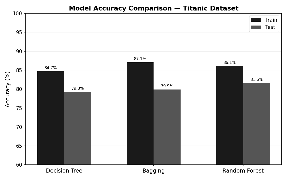
All three models use max_depth=5. Random Forest achieves the highest test accuracy at 81.6%, beating the single Decision Tree (79.3%) and Bagging (79.9%). The gap between train and test bars shows how much each model overfits.
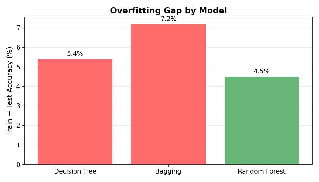
The train−test accuracy gap measures how much each model memorizes vs. generalizes. Decision Tree: 5.4 pp. Bagging actually widens it to 7.2 pp because its highly correlated trees all overfit in the same direction. Random Forest closes it back down to 4.5 pp by decorrelating the trees, giving it the tightest gap of the three.
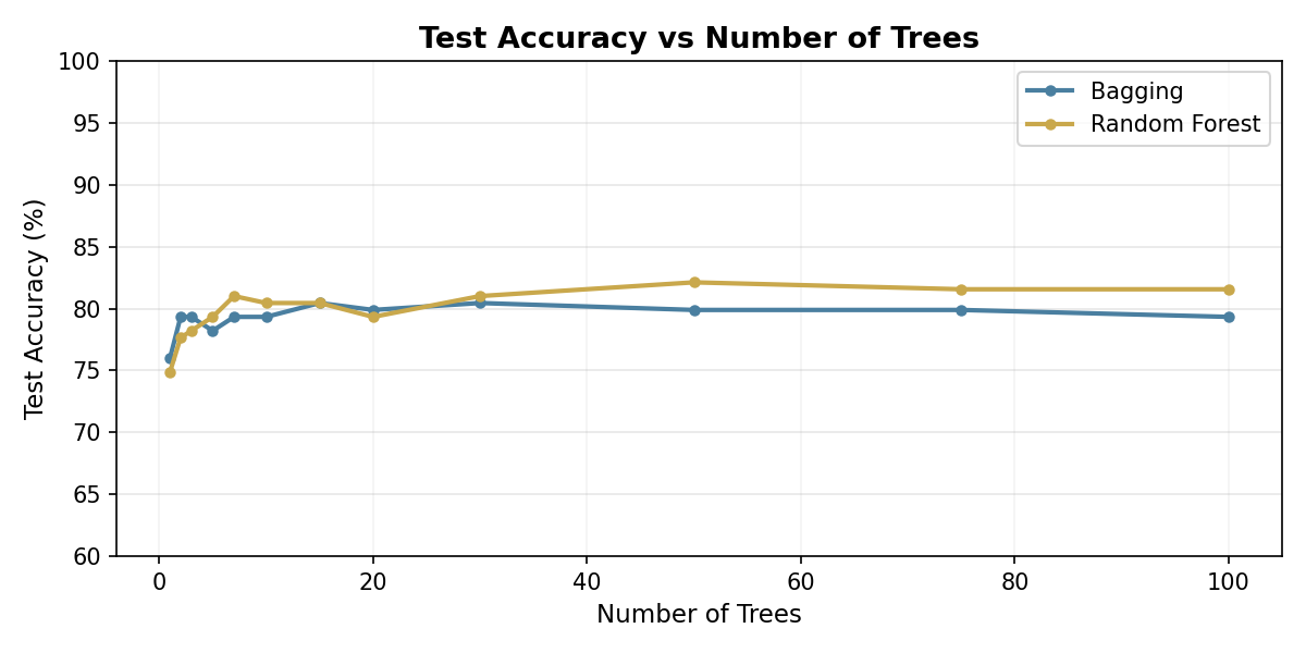
Both methods improve quickly, then flatten out. The reason is mathematical: the variance of a B-tree ensemble is Var = ρσ² + (1−ρ)σ²/B. The second term shrinks as you add trees, but the first term, ρσ², is a hard floor that no number of trees can remove. At 10,000 trees the second term is essentially zero, but accuracy still cannot exceed the ceiling set by that floor. The only way past it is to lower ρ, the correlation between trees. That is exactly what Random Forest does: by forcing each split to see only a random subset of features, its trees disagree more often, ρ drops, and the floor is lower. Bagging never reduces ρ because every tree can use every feature, so it levels off below Random Forest. A Decision Tree is a single tree by definition and is not shown.
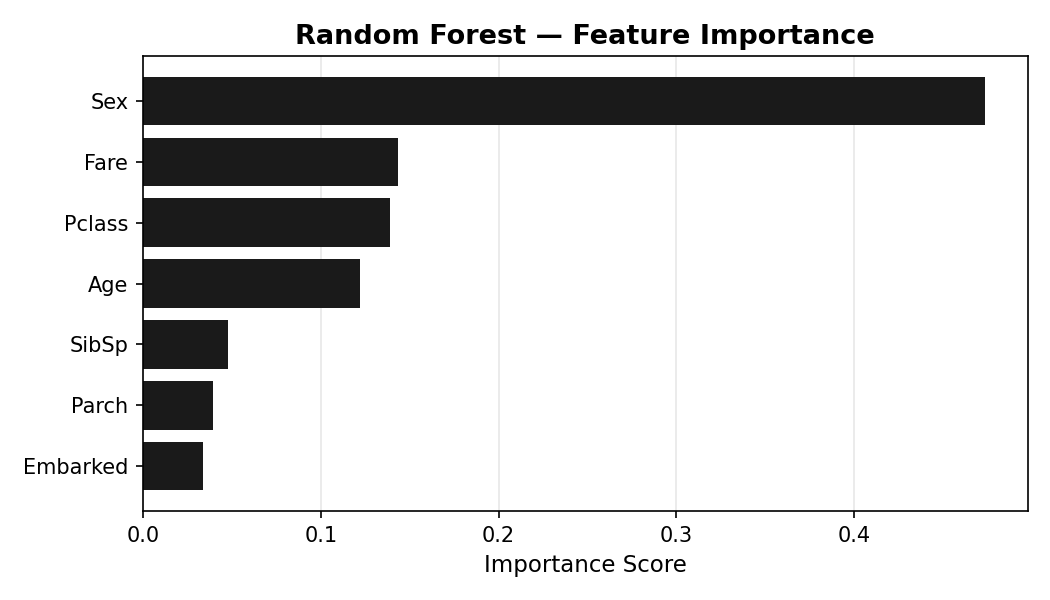
Sex is by far the strongest predictor of survival, consistent with historical accounts of "women and children first." Passenger class and fare, both proxies for socioeconomic status, rank second and third. Age contributes meaningfully; port of embarkation contributes very little.
Ensembles are generally the stronger choice, but understanding your data before applying a model matters just as much as the model itself. Bagging underperformed here not because it is a weaker method, but because this dataset has a few heavily weighted features: sex, class, and age dominate survival prediction. When every tree sees all features, they all split on the same signals and stay correlated. Random Forest forces diversity by restricting what each split can see, which is why it pulls ahead.
The lesson is not just that Random Forest wins. It is that knowing why it wins, and when it would not, is what makes the difference between applying a tool and understanding one.